Ray Tracer Challenge, pt. 2: Enter The Matrix

March 2, 2023

tags: algorithms, graphics, math, ray-tracer-challenge, rust

The full code for this challenge can be found at this repo.

Welcome back! Last time we set up the foundational data structures for our ray tracer by creating points, vectors, colors, and the canvas on which to draw them. This time, we’re going to continue with a very important foundational concept: the matrix. We’ll be able to transform shapes in our image by multiplying them with specific matrices. This will entail modeling some linear algebra magic with algorithms, but don’t worry if that sounds scary; matrix manipulations are pretty straightforward.

It’s That Time Again

Like in part one, let’s start at the end and see our rewarding image:

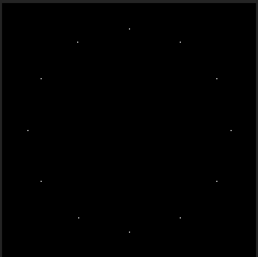
Wow. Mind blowing, right? It may not be a ray traced Mona Lisa, but it showcases some of the bread and butter calculations that we’ll need to make much more impressive scenes later on. This example takes an initial point and transforms it to create new points showing where every hour sits on an analog clock. Here’s the code used to generate this image:

use std::f64::consts::PI;
const RADIANS_IN_AN_HOUR: f64 = PI / 6.0;

fn main() {
    let mut canvas = Canvas::new(250, 250);
    let start_point = Tuple::point(0.0, -100.0, 0.0);

    for hour in 1..=12 {
        let transformation = Matrix::identity()
            .rotate_z(hour as f64 * RADIANS_IN_AN_HOUR)
            .translate((canvas.width / 2) as f64, 125.0, 0.0);
        let new_point = transformation * start_point;
        canvas.write_pixel(&new_point, Color::white());
    }

    save_image(canvas);
}

Side note: I refactored the Point and Vector structs into one Tuple struct with named constructors: ::point and ::vector. This cleaned up a lot of duplicated code and simplified the whole design since we only need to think about the one type.

At a high level, we take the starting point, rotate it across the Z axis, then move it along the X and Y axes (translation). This is done for every hour: 1..=12 inclusive range. Each new point is then written to the canvas before the whole thing is converted to PPM format and saved to disk (review in part one). The main change to note here is the use of the new Matrix type, which we’ve so eloquently implemented with a fluent interface.

Red pill or blue pill?

So, WTF is a matrix? It’s a grid of numbers. Boom. Here’s some examples:

For ray tracing, we’ll mostly use 4x4 matrices. To implement this, we’ll opt for a simple approach and just use a vector of vectors (unlike how the Canvas works with a single vector).

pub struct Matrix {
    rows: Vec<Vec<f64>>,
}

impl Matrix {
    fn populate(rows: Vec<Vec<f64>>) -> Self {
        Self { rows }
    }
}

let matrix = Matrix::populate(vec![
    vec![8.0, -5.0, 9.0, 2.0],
    vec![7.0, 5.0, 6.0, 1.0],
    vec![-6.0, 0.0, 9.0, 6.0],
    vec![-3.0, 0.0, -9.0, -4.0],
]);

Something really cool we can do with this Matrix type allow it to handle indexing:

impl Index<usize> for Matrix {
    type Output = Vec<f64>;

    fn index(&self, index: usize) -> &Self::Output {
        &self.rows[index]
    }
}

impl IndexMut<usize> for Matrix {
    fn index_mut(&mut self, index: usize) -> &mut Self::Output {
        &mut self.rows[index]
    }
}

The first implementation returns an immutable reference to a row from the matrix: matrix[2]. Then, it’s just indexing that vector as usual to get the value for the column: matrix[2][0]. The second method returns a mutable reference, which allows us to set values in the matrix through indexing: matrix[6][15] = 1.8. This is super cool!

Who Am I?

The next thing we want out of Matrix is its identity. When you multiply any number by 1 you get the original number back. This makes 1 the multiplicative identity. The equivalent for matrices is a matrix which when multiplied by another matrix or tuple returns that matrix or tuple.

// 4x4 identity matrix
impl Matrix {
    pub fn identity() -> Self {
        Self::populate(vec![
            vec![1.0, 0.0, 0.0, 0.0],
            vec![0.0, 1.0, 0.0, 0.0],
            vec![0.0, 0.0, 1.0, 0.0],
            vec![0.0, 0.0, 0.0, 1.0],
        ])
    }
}

We Don’t Die, We Multiply

Now that we have the identity, we need to know how to actually multiply matrices with themselves and tuples. The product of two matrices is another matrix. Let’s look at an example:

   A             B             C
 1 2 3 4     (0) 2  4  6    [] [] [] []
(2 3 4 5)    (1) 2  4  8    31 [] [] []
 3 4 5 6  X  (2) 4  8 16  = [] [] [] []
 4 5 6 7     (4) 8 16 32    [] [] [] []

To calculate the value of an element in the product, C[1, 0] in this case, you multiply the corresponding row in A[1, col] with the column in B[row, 0] and then sum them together.

2 * 0 = 0
3 * 1 = 3
4 * 2 = 8
5 * 4 = 20
0 + 3 + 8 + 20 = 31

In Rust speak:

impl Mul for &Matrix {
    type Output = Matrix;

    // Assumes the rows are of equal length
    fn mul(self, other: &Matrix) -> Self::Output {
        let mut product = self.clone();
        let width = self.rows[0].len();

        for row in 0..width {
            for col in 0..width {
                let mut sum = 0.0;
                for idx in 0..self.rows.len() {
                    sum += self[row][idx] * other[idx][col]
                }
                product[row][col] = sum;
            }
        }
        product
    }
}

// Implementing Mul let's us do this. It returns a new matrix. Pretty neat.
let product = matrixA * matrixB;

A possible problem I see with this code is the left hand side matrix is moved into the mul method and dropped. We won’t ever be able to work with that matrix again. We don’t know what the future of our ray tracing matrix manipulations entail, so this has the potential to be an issue later on. Put a pin in that.

Multipling a matrix with a tuple is nearly the same, but you only have one column on the right hand side and a tuple is returned.

   A          B       C
 1 2 3 4     (0)     []
(2 3 4 5)    (1)     31
 3 4 5 6  X  (2)  =  []
 4 5 6 7     (4)     []

Here’s our beautiful, smelly, hardcoded Rust representation.

impl Mul<Tuple> for Matrix {
    type Output = Tuple;

    // Hardcoded for a 4x4 matrix
    // This could be cleaned up if Tuple were iterable.
    fn mul(self, other: Tuple) -> Self::Output {
        let x = self[0][0] * other.x
            + self[0][1] * other.y
            + self[0][2] * other.z
            + self[0][3] * other.w;
        let y = self[1][0] * other.x
            + self[1][1] * other.y
            + self[1][2] * other.z
            + self[1][3] * other.w;
        let z = self[2][0] * other.x
            + self[2][1] * other.y
            + self[2][2] * other.z
            + self[2][3] * other.w;
        let w = self[3][0] * other.x
            + self[3][1] * other.y
            + self[3][2] * other.z
            + self[3][3] * other.w;
        let mut point = Tuple::point(x, y, z);
        point.w = w;
        point
    }
}

let new_point = matrix * point;

We can think of these matrices as transformations we can apply to points to create new points. The identity matrix doesn’t change anything by itself; it is simply a starting point to be tweaked into different transformations. To complete our analog clock, we need two more tweaks: rotation around the Z-axis and moving a point to a different location, called translation. Let’s start with the latter.

Lost In Translation

We have a point (0, 1, 0), and we need to move it to (20, 30, 40) by multiplying it with a translation matrix. We do this by setting the tuple’s X to the identity matrix’s [0, 3], Y to [1, 3], and Z to [2, 3].

Now we can move points around!

pub fn translate(&self, x: f64, y: f64, z: f64) -> Self {
    let mut transform = Matrix::identity();
    transform[0][3] = x;
    transform[1][3] = y;
    transform[2][3] = z;
    &transform * self
}

let point = Tuple::point(0.0, 1.0, 0.0);
// This returns (20, 30, 40)
let new_point = matrix.translate(20.0, 29.0, 40.0) * point;

We can multiply a reference to a matrix with a reference to another matrix because we specified those types in the trait implementation: impl Mul for &Matrix.

The final piece we need to make our analog clock tick is Z-axis rotation. To help you picture this, stand straight and raise your arms parallel to the ground pointing away from you like a T. Your arms are the X axis, your body is the Y axis, and Z is a line shooting out of your chest straight ahead of you. This makes your heart the origin. Awwwwww. We want our point to rotate clockwise around this chest line to create a circle. This means the Z axis will always remain 0, and X and Y are the ones that change. And since we’re talking about circles, math showed up and brought some Pi. That math is so nice.

She’s My Cherry Pi

Rotation involves moving a point by an angle relative to the origin point on the other end of the line. Circles and angles everywhere means our friend Trigo Nometry was invited to the party. There is some hand waving at this point because I don’t know how this actually works, but it does. These mathy matrices are provided by the book, and each axis needs its own to represent rotation. The matrix specifically needed for the Z-axis is as follows:

cos(r) -sin(r) 0 0
sin(r) cos(r)  0 0
0      0       1 0
0      0       0 1

The cosine, sine, and negative sine of the given radians (r) are set in these specific positions. Radians are a measurement of the curved distance between two points. Below is a visual example. Don’t be jealous of my Paint skills.

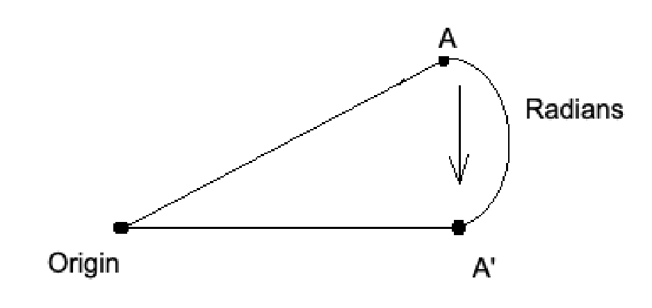
A full cirle (360˚) has 2π radians, so half (180˚) is π radians. Rust is so friendly, that it implements trigonometric methods directly on numbers! We don’t even need to import a math library.

pub fn rotate_z(&self, radians: f64) -> Self {
    let mut transform = Matrix::identity();
    transform[0][0] = radians.cos();
    transform[0][1] = -radians.sin();
    transform[1][0] = radians.sin();
    transform[1][1] = radians.cos();
    &transform * self
}

We’ll have 12 o’clock be our starting point. Going from there to 3 on a clock is a quarter circle, π/2 radians (2π/4). However, the distance of each hour is a third of that because there are three hours in a quarter. Since 2*3 == 6, the distance in radians for an hour would be π/6. As an example, to calculate a matrix that rotates a point from 12 to 7, you would need 7 of those one hour distances:

const RADIANS_IN_AN_HOUR: f64 = PI / 6.0;
let matrix = matrix.rotate_z(7.0 * RADIANS_IN_AN_HOUR);

Have I Mentioned I’m Fluent In Interfacing?

Let’s bring it back to the final code that generates the clock canvas and walk through it now that we know more about it.

let mut canvas = Canvas::new(250, 250);
let start_point = Tuple::point(0.0, -100.0, 0.0);

for hour in 1..=12 {
    let transformation = Matrix::identity()
        .rotate_z(hour as f64 * RADIANS_IN_AN_HOUR)
        .translate((canvas.width / 2) as f64, 125.0, 0.0);
    let new_point = transformation * start_point;
    canvas.write_pixel(&new_point, Color::white());
}

We create a square canvas and start with an origin point at (0, -100). Remember, the canvas begins at the upper left corner, so a negative Y value will put the point above the canvas. For each hour, we rotate on Z to move the point π/6 radians, then translate that point halfway across (250/2 + X) and 25 down (125 + Y) the canvas. Calculate the appropriate matrix and multiply it with the point to create a new point. Voila.

One aesthetic point I like that the book mentions is providing a fluent interface for the Matrix type. We start with the identity, then transform it with a rotation, then transform that with a translation. This fluent method chaining allows for a pipelined form of state transitions by taking the initial receiver, modifying it, and then returning it. In our implementations, we’re dealing with immutable references, so the matrix returned is a new instantiation, rather than the same struct modified. This could have performance concerns down the line, but we should always wait to cross that bridge when we get there. “Premature optimization is the root of all evil,” said a smart person somewhere.

Final Summation

I’ll admit I never took linear algebra in college, so I would not have come up with these specific matrices on my own without a lot of research. Why do we need those specific trig functions in those specific places in a matrix in order to properly manipulate points on a grid? Don’t ask me. What I do understand is the beauty of watching it work when applied. We seem to have most of the foundation of our ray tracer at this point. In the next chapter, we’ll actually be creating rays and shooting them at spheres. If that doesn’t sound exciting, then I don’t why you’re reading this. But I still appreciate you. Until then.

Notes

The radians painting masterpiece created at jspaint.app