Ray Tracer Challenge, pt. 1: Creating A 2D Image

January 10, 2023

tags: algorithms, graphics, ray-tracer-challenge, rust

The full code for this challenge can be found at this repo.

Hello there! Have you ever wondered what goes on under the hood when generating computer graphics? Ever yearned to write a 3D renderer from scratch? Me too! You’ve come to the right place, my friend. This is the first in a series of posts detailing my adventures in doing just that. A ray tracer, specifically. And my guide on this journey is the incredible book The Ray Tracer Challenge.

It’s fantastic! This book is how all tutorials should be structured. Each chapter builds on the previous, describing what needs to be implemented in order to create a program that has the power to generate 3D images. The killer feature is that you can code it however you want. There are no copy pastas or typing exercises involved. You’re given explanations of what must be done and high level tests to prove it works. You are free to use whatever you can to get the tests to pass and have a running program. So cool. If you’ve read any of my recent posts, you’ll correctly guess that I chose Rust to complete this challenge. As an extra bonus, a ray tracer is a non-trivial piece of work that will get you deep into your chosen tech, which makes it a way to apply a language you are learning.

Show Me Something

Part one is about laying the foundation for our renderer. Before we can get to making amazing 3D images, we need to start with making amazing 2D images. Along the way we’ll develop some of the primitive structures that our ray tracer will need to work. Let’s skip straight to the end to see our reward:

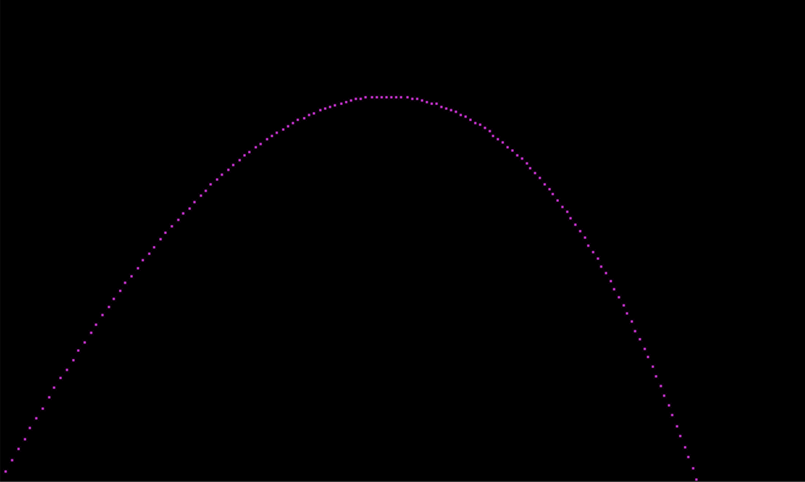
It’s beautiful! We launched a projectile from the bottom left corner of the image with a given velocity. It fights through wind and gravity to screech into the sky before it’s finally overcome and begins its descent, landing somewhere on the right. How cool is that? It’s like the Hello World of rendering.

What’s Your Point?

From that description, we can identify several entities we’ll need to model. Let’s start with the most fundamental. Looking at the image, we see it’s simply a collection of points at different positions on a grid. A 2D point is a coordinate on the X and Y axes: (1.0, 3.2). Our first codes!

struct Point {
    x: f64, // x-axis
    y: f64, // y-axis
    z: f64, // z-axis for when we go 3D
    w: f64, // special value denoting a Point
}

impl Point {
    pub fn new(x: f64, y: f64, z: f64) -> Self {
        Self { x, y, z, w: 1.0 }
    }
}

let point = Point::new(4.0, 3.2, 0.7); // 3D point

We’ve gone ahead and added a field for the z-axis, technically making this a 3D point. The book describes a point as a four element tuple where the “w” field is 1 (types are an implementation detail that the book is unconcerned with). Beyond specifying a type, the “w” value will be important later on when we need to multiply matrices. We’re also using floating point numbers here so that we can be as precise as possible!

Tick Tock

Now that we have a point, we must figure out how to make it change over time to create a trajectory. Let’s lay the foundation with a loop and the famous gaming tick function. Each tick will evaluate the state of the world and transform the point accordingly. The loop should stop when the point’s Y value reaches 0, which means it’s lying on the ground.

let mut point = Point::new(0.0, 0.0, 0.0);

while point.y > 0.0 {
    point = tick(point);
}

fn tick(point: Point) -> Point {
    point
}

Ship it! Well, this begs the question of how do we change a point? With a vector!

How Vexing

Vectors (no, not Rust vectors) are just the lines between points. Given points (1, 2) & (3, 4), the vector would be (2, 2). It describes the direction and distance the first point needs to move to become the second. Adding a vector to a point will produce this “moved” point, which is exactly what we need. We can model it the same as a Point, but set the “w” to 0.0.

struct Vector {
    x: f64,
    y: f64,
    z: f64,
    w: f64,
}

impl Vector {
    pub fn new(x: f64, y: f64, z: f64) -> Self {
        Self { x, y, z, w: 0.0 }
    }
}

This next part is cool and reminds me of Python’s object model. How do we add a point and a vector? Overload the addition operator by implementing the std::ops::Add trait.

impl Add<Vector> for Point {
    type Output = Self;

    fn add(self, other: Vector) -> Self {
        Self {
            x: self.x + other.x,
            y: self.y + other.y,
            z: self.z + other.z,
            w: self.w + other.w,
        }
    }
}

let new_point = point + vector;

Add is generic over the right hand side (Add<Rhs = Self>). By implementing add for Point and declaring the right hand side as a Vector, we can add a vector to a point. However, the opposite won’t work: vector + point. We’d need to do the same for Vectors and define impl Add<Point> for Vector to have commutativity. Since the generic type defaults to Self, you can leave it out and add Points to Points or Vectors to Vectors with impl Add for Vector.

What Projects Are You Working On?

A point and a vector compose a projectile, where the point is its position and the vector is its velocity.

struct Projectile {
    position: Point,
    velocity: Vector,
}

For each tick, the projectile’s position can be transformed by applying its velocity.

fn tick(projectile: Projectile) -> Projectile {
    Projectile {
        position: projectile.position + projectile.velocity,
        velocity: projectile.velocity
    }
}

This code works great if you want to see a projectile shoot into space on a linear trajectory. We neet to make the velocity change so we’re not just drawing a straight line. We could go crazy here modelling an environment with all sorts of physical aspects, but let’s keep it simple and provide gravity to bring the projectile back down to earth and wind just to annoy the velocity. We’ll also keep it immutable, so the environment never changes.

struct Environment {
    gravity: Vector,
    wind: Vector,
}

fn tick(env: &Environment, projectile: Projectile) -> Projectile {
    Projectile {
        position: projectile.position + projectile.velocity,
        velocity: projectile.velocity + env.gravity + env.wind,
    }
}

And now the updated generation of a trajectory:

let env = Environment {
    gravity: Vector::new(0.0, -0.1, 0.0), // negative Y to push down
    wind: Vector::new(-0.01, 0.0, 0.0), // negative X to add resistance
};

let mut projectile = Projectile {
    position: Point::new(0.0, 1.0, 0.0),
    velocity: Vector::new(1.0, 1.8, 0.0), // magic numbers, AKA machine learning params
};

while projectile.position.y > 0.0 { // not heavy enough to bore into the Earth
    projectile = tick(&env, projectile);
    // do something to record this state
}

We start the position just off the ground, so the loop will actually run (also to account for the height of the launcher, am I right?). Gravity and wind are both negative so as to gradually drop and slow the projectile. The velocity and environment values are highly tweakable and perfect for experimenting with different results. The book goes into vector magnitude, normalization, and multiplication in order to create a nice trajectory curve. I’m glossing over those details for now, so if you’re interested, get the book!

Do You Dream In Color?

We’ve implemented changing points over time, but we’re not doing anything with them, yet. Our points long to be dropped onto a grid, which will then become the canvas that we’ll paint. But what does a point even look like? We need to introduce some color. The canvas will be black to start with (cause dark mode is cool) and our point will be purple because its my wife’s favorite color.

One way to represent color is varying shades of red, green, and blue. If we model these values on a range between 0 and 1, we can represent an infinite scale of colors. Since white light can be broken up into its component colors through a prism, it can be modeled as the maximum of all three RGB colors: (1,1,1). On the other hand, the absence of color is black (0,0,0).

struct Color {
    red: f64,
    green: f64,
    blue: f64,
}

impl Color {
    pub fn new(red: f64, green: f64, blue: f64) -> Self {
        Self { red, green, blue }
    }

    pub fn black() -> Self {
        Self::new(0.0, 0.0, 0.0)
    }

    pub fn white() -> Self {
        Self::new(1.0, 1.0, 1.0)
    }
}

Eventually, we’ll need to convert these floats to a bounded scale that can be practically used. The human eye can’t tell the difference between a red at 0.555555555555 and one at 0.555555555556. Also, the image spec we’re going to use for saving the canvas to a file doesn’t handle values like that. But more on that later.

Let’s make the scaled range start at 0 and max out at 255 (because the book says so). In order to scale a number in the range of 0.0 to 1.0, we need to multiply it with the total number of values, 256 in this case. Also we should constrain the result not to go below 0 or above 255. Et voila:

fn scale_color(color: &Color, max: i32) -> [i32; 3] {
    let total_values = (max + 1) as f64; // include 0 (0..=max is max+1 values)
    [color.red, color.green, color.blue].map(|value| {
        let scaled = (value * total_values) as i32;
        scaled.clamp(0, max) // thanks Rust!
    })
}

let pink = Color::new(0.5, 0.0, 0.0);
assert_eq!(scale_color(pink, 255), [128, 0, 0]);

It’s A Blank Canvas

Our canvas of pixels is implemented as a grid of points. My favorite way to code a 2D grid is with a contiguous array. For example, let’s take a 5x5 grid. It contains 25 points, which can be held in a 25 element array. The first element is the top left corner of the grid, so the corresponding indexes would hold the individual points:

0  1  2  3  4
5  6  7  8  9
10 11 12 13 14
15 16 17 18 19
20 21 22 23 24

A point is a pixel, and a pixel is just a color. When a new canvas is created, it will default to black, so load up its pixel array with black colors.

pub struct Canvas {
    width: i32,
    height: i32,
    pixels: Vec<Color>,
}

impl Canvas {
    pub fn new(width: i32, height: i32) -> Self {
        let capacity = width * height; // capacity is known!
        let mut pixels = Vec::with_capacity(capacity as usize); // allocate list
        for _ in 0..capacity {
            pixels.push(Color::black()); // fill list with black pixels
        }

        Self {
            width,
            height,
            pixels,
        }
    }
}

Pixelation

We have a canvas! Remember when we used the tick function? Now, after each tick, we can write a purple pixel into the canvas corresponding to the point of the projectile.

let mut canvas = Canvas::new(500, 300);

while projectile.position.y > 0.0 {
    projectile = tick(&env, projectile);
    let position = projectile.position;
    let pos_y = canvas.height - (position.y as i32); // flip Y
    if pos_y <= canvas.height {
        let pixel = Color::new(1.0, 0.0, 1.0); // red and blue make purple
        canvas.write_pixel(position.x as i32, pos_y, pixel);
    }
}

A couple gotchas: the projectile’s Y coordinate is upside-down because the canvas’s origin is the top left, not the bottom left. Y increases as you travel down the canvas. To handle this, we need to flip the projectile’s Y value by subtracting it from the height of the canvas. Also, we won’t write pixels if the projectile falls off the canvas. We could also check X and maybe even move that logic into the canvas module itself.

Writing a pixel simply consists of putting it into the canvas’s vector of pixels. The neat thing is determining how to find the proper index. Striding is a way to convert a point to an index within a grid. Remember our example grid:

0  1  2  3  4
5  6  7  8  9
10 11 12 13 14
15 16 17 18 19
20 21 22 23 24

Given point (3,2), the index would be 13. The formula to find this is y * width + x.

(3,2) -> 2*5+3 = 13
(0,4) -> 4*5+0 = 20
(4,1) -> 1*5+4 = 9

Pretty cool! I learned this trick from reading Hands-on Rust. That’s also a great book, though it’s more focused on game development than Rust itself. The Ray Tracer Challenge does not mention this formula. I’ll say it again, the thing I enjoy the most about it is it doesn’t spell out how to implement anything. It’s totally up to you.

Now that we know how to put a point into a vector (yes, Rust vectors), let’s do it!

pub fn write_pixel(&mut self, x: i32, y: i32, pixel: Color) {
    let idx = self.point_to_index(x, y);
    if idx < self.pixels.len() { // ignore if index is out of bounds
        self.pixels[idx] = pixel;
    }
}

You may notice there is no check for a negative index. The compiler makes that unnecessary because vectors can only be indexed with unsigned integers.

Save Your Work!

We now have a canvas painted with the trajectory of a projectile. The final piece of work is to convert that in-memory data into an file saved on disk. That way we can open and view it at our leisure. What type of file should we use? One I had never even heard of before this book: PPM! The Portable Pixmap is just one of many ways to encode graphics formats. It consists of a header and pixel data:

P3
5 3
255
255 0 0 0 0 0 0 0 0 0 0 0 0 0 0
0 0 0 0 0 0 0 128 0 0 0 0 0 0 0
0 0 0 0 0 0 0 0 0 0 0 0 0 0 255

The first three lines are the header:

P3 - The PPM spec. P3 means “plain” PPM.
5 3 - Image width and height in pixels.
255 - Maximum color value - each red/green/blue value can be 0-255.

The rest is the representation of pixels in the image. The height is 3, so there are 3 lines. Each pixel contains values for 3 colors (red, green, blue) and the width is 5. Therefore, each line has 3*5 integers that don’t exceed the max value (255), seperated by spaces. Logically grouping the pixels can help you visualize:

(255 0 0) (0 0 0) (0 0 0) (0 0 0) (0 0 0)

To convert the canvas to a PPM file, write the header to a string then iterate over the pixels and stringify them before appending. Don’t forget to scale the color values! Also, PPMs have a line length limit of 70; the rest of the grid row will be put on a new line. Here’s a first iteration that gets slow very quickly for bigger canvases. I’m sure I’ll need to optimize it as I get further along in the book, which will be fun in and of itself. I’ve always enjoyed the algorithms part of coding the most. Everything else is just boilerplate.

const MAX_PPM_VALUE: i32 = 255;
const PPM_LINE_SIZE: i32 = 70;

// Color values are scaled bewteen 0 and 255: 0:0-1:255
// This algorithm runs pretty slow.
// At 500x300 canvas: "cargo run  7.40s user 4.33s system 99% cpu 11.822 total"
pub fn to_ppm(&self) -> String {
    let mut ppm = format!("P3\n{} {}\n{}\n", self.width, self.height, MAX_PPM_VALUE);
    let scaled_pixels: Vec<[i32; 3]> = self
        .pixels
        .iter()
        .map(|color| scale_color(color, MAX_PPM_VALUE))
        .collect();

    for chunk in scaled_pixels.chunks(self.width as usize) {
        let mut char_count = 0;
        let color_values = chunk.iter().flatten().map(|values| values.to_string());
        for value in color_values {
            let next_char_count = char_count + value.len() as i32 + 1; // for the space
            if next_char_count > PPM_LINE_SIZE {
                ppm.pop();
                ppm = format!("{}\n{} ", ppm, value);
                char_count = 0;
            } else {
                ppm = format!("{}{} ", ppm, value);
                char_count = next_char_count;
            }
        }
        ppm.pop();
        ppm.push('\n');
    }
    ppm
}

Now we have the text version of our image! Save it to a file.

let mut file = File::create("images/trajectory.ppm").unwrap();
file.write_all(canvas.to_ppm().as_bytes()).unwrap();

There are various apps you can use to render a .ppm file. On macOS, Preview.app has built-in support. In Linux, you can use GIMP. And there you have it!

Final Summation

This turned out to be a heavier, longer post than I anticipated, but I still think it’s interesting enough to read, although you are the real judge of that. It must have been, if you’re still here. I’m excited to dig more into the book and get closer to rendering amazing 3D images. Once I feel like I’ve learned enough to warrant one, I’ll write the next post in the series. See you then!